Unique Eccentricity Profiles

Unique eccentricity profiles refer to profiles where eccentricity is a unique function of semi-major axis, \(e = e(a)\), which can also be written as \(\psi(e, a) = \delta(e - e(a))\). Such eccentricity profiles are defined through the UniqueEccentricity class.

Initialising the UniqueEccentricity Class

When initialising the eccentricity class, the user must firstly supply the a_min and a_max values, defining the range of semi-major axes.

In terms of the profile being used, there are two ways to initialise the class:

1. Using the built-in power-law profile,

   \[e(a) = e_0 \left(\frac{a_{\min}}{a}\right)^{p}\]

2. Providing a custom function,

\[e(a) = e_0 \cdot e(a)_\text{custom}\]

In both cases, the class automatically checks that the returned eccentricities lie within the physically valid range \(0 \leq e(a) < 1\).

Unlike the SigmaA class, the eccentricity is not truncated outside of \([a_{\min}, a_{\max}]\). The UniqueEccentricity class is primarily a lightweight, object-oriented wrapper for storing and evaluating \(e(a)\), and is designed for direct use with the Kernel class when computing the ASD.

Built-In Eccentricity Profile

The class defaults to the built-in power-law profile, for which the user must define the scaling factor, e0, and the power argument.

# Import the class
from debrispy import UniqueEccentricity
import numpy as np

# Initialise
power_law = UniqueEccentricity(a_min=1, a_max=4, e0=0.5, power=0.5)

Custom Eccentricity Profile

Alternatively, the user can override the power law profile by supplying their own function through the eccentricity_func argument. Even in this case, the user is free to define the normalisation, e0, which defaults to 1 if unspecified.

⚠️ Important: If providing a custom eccentricity function, it should be vectorised (so scalar Python conditionals such as if/else will usually fail, use NumPy-aware operations instead), and be provided in such a way that the semi-major axis, \(a\), is the only parameter. This can be done by wrapping the function manually or using a lambda function.

def ecc(a, b, c):
    return np.abs(np.sin(a*b))*c

custom = UniqueEccentricity(a_min=1, a_max=4, e0=1,
                            eccentricity_func=lambda a: ecc(a, b=0.5, c=0.5))

Returning Eccentricity Values & Profile Information

Profile information can be obtained via the print functionality.

print(power_law)
print(custom)

UniqueEccentricity(a_min=1, a_max=4, e0=0.5, power=0.5)
UniqueEccentricity(a_min=1, a_max=4, e0=1,  custom_func=True)

One can evaluate the eccentricty at specific a values, either by calling the eccentricity method, or by simply calling the class as a function (which internally also uses the same method).

a_vals = [2, 2.5, 3]
print(power_law(a_vals))
print(power_law.eccentricity(a_vals))

[0.35355339 0.31622777 0.28867513]
[0.35355339 0.31622777 0.28867513]

Calculating the Derivative

In addition, the class contains a derivative method to calculate \(de/da\). This is not directly part of the ASD pipeline, however can be an effective way to determine or visualise sharply peaked regions. This is calculated for arbitrary eccentricity distributions numerically using the central differences method.

a_vals = [1, 2, 3, 4]
custom_profile_derivatives = custom.derivative(a_vals)
print(custom_profile_derivatives)

[ 0.21939564  0.13507558  0.0176843  -0.10403671]

Visualising the Eccentricity Profile

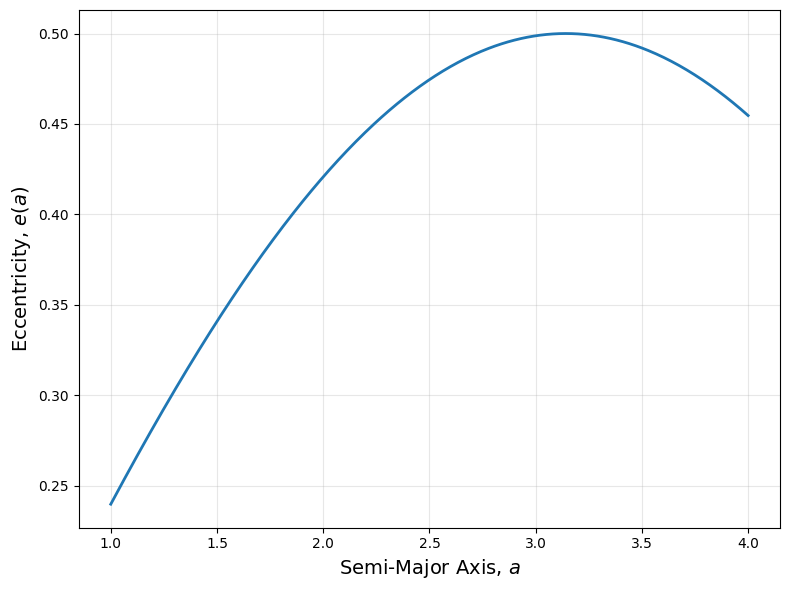
The plot() method of the UniqueEccentricity class provides a flexible interface for visualising the eccentricity profile.

By default, it will:

• Generate 500 points uniformly in the interval \([a_{\min}, a_{\max}]\)

• Plot ( e(a) ) on linear axes

• Label the axes and show a grid

• Display the figure unless save=True is specified (note that filename must be provided if save=True)

custom.plot()

Some useful keyword arguments include:

Plot appearance:

• color: Line colour (e.g. 'k', 'C1', '#FF0000')

• linestyle: '-', '--', ':', etc.

• linewidth or lw: Line width

• marker: Marker style ('o', '.', 's', etc.)

• alpha: Line transparency

• label: Legend label

Axes and layout:

• xlim, ylim: Axis ranges

• xlabel, ylabel, title: Override axis labels and title

• grid: Show/hide grid

• log: If True, use log scale for y-axis

• save=True, filename="...": Save figure instead of displaying

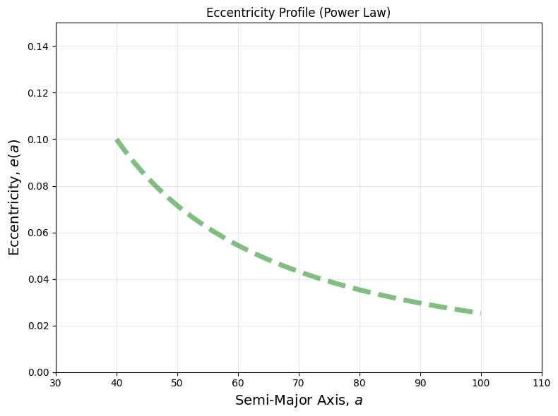
ecc = UniqueEccentricity(a_min=40, a_max=100, e0=0.1, power=1.5)

ecc.plot(
    color='green',
    linestyle='--',
    linewidth=5,
    alpha=0.5,
    xlim=(30, 110),
    ylim=(0, 0.15),
    title='Eccentricity Profile (Power Law)',
    grid=True
)