Using the SigmaA Class

The surface density with respect to semi-major axis, \(\Sigma(a)\) is defined through the SigmaA class. This class must be initialised for the pipeline, and is directly used when computing the final \(\bar\Sigma(r)\) profile.

The class comes with a host of pre-built \(\Sigma(a)\) profiles but also supports any supplied functional form. This page demonstrates all of the built in functionalities within the class.

Getting Started: Class Functionality

To begin using the class, the user must first initialise it by specifying the following:

• The minimum and maximum semi-major axes, set via the a_min and a_max arguments (these define the truncation bounds)

• The overall amplitude or normalisation factor, specified using sigma0

• The desired profile type, selected through the profile_type argument

In addition to these required parameters, each built-in profile type accepts its own specific keyword arguments, which must also be supplied at initialisation. These profile-specific arguments are summarised in the table below and explained in more detail in the following sections:

Profile Type	Required Parameters
'power_law'	power
'gaussian'	gauss_width, gauss_center
'step_up'	step
'step_down'	step
'custom'	custom_func (callable)

Initialising the Class

This is an example on how to initialise the class with a power-law profile. Each built-in profile has its own arguments that must be defined. See the next sections for demonstrations with the other built-in profiles. In the case of the power-law, the user must define the power parameter.

# First import the class
from debrispy import SigmaA
import numpy as np

# Initialise
sigma_a_profile = SigmaA(a_min=1, a_max=4, profile_type='power_law', sigma0=1, power=0.5)

Getting Information about the Class via Print

Once initialised, the user can get check information about the class parameters, such as the profile type and semi-major axis range, by simply printing the class.

print(sigma_a_profile)

SigmaA(type=power_law, a_min=1, a_max=4, sigma0=1, power=0.5)

Calculating and Returning the \(\Sigma(a)\) Values

Once initialised, the user can obtain the \(\Sigma(a)\) values for a chosen array of \(a\) values by using the get_values method or by simply calling the class as a function, which internally uses the same method.

# Define the a values to calculate the profile over
a_vals = np.linspace(0.01, 4, 5)

# Option 1: Return the values through the 'get_values' method
sigma_a_vals = sigma_a_profile.get_values(a_vals)

# Option 2: Return the values by calling the initialised class directly
sigma_a_vals = sigma_a_profile(a_vals)

print(sigma_a_vals)

[0.         0.99627096 0.70622455 0.57710986 0.5       ]

Visualising the Profile

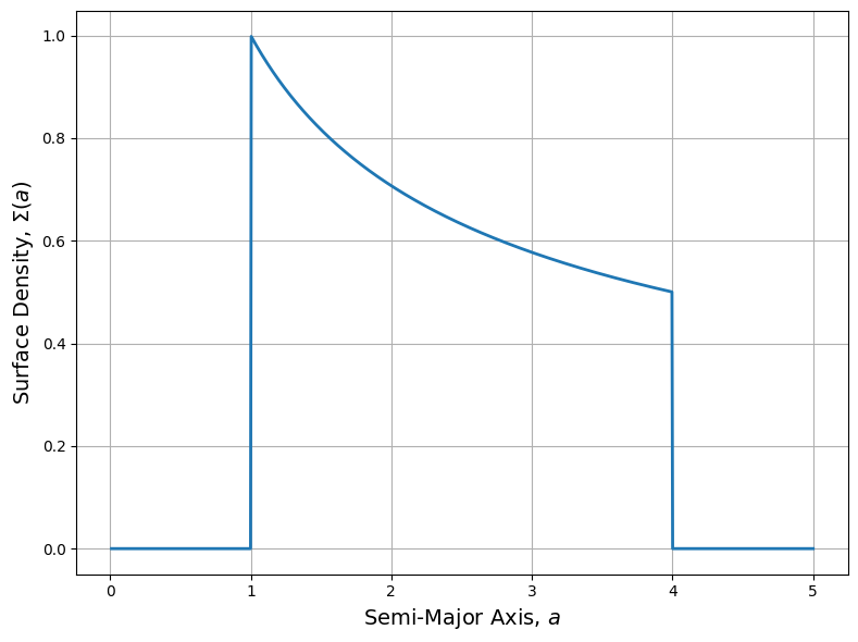
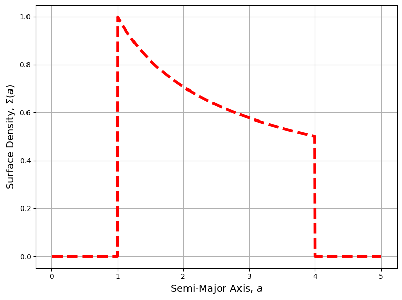
The Sigma(a) class also a plotting tool, which can be called through the plot method. This method has a host of arguments to change appearance of the plot, and also has support for any plt.plot keyword arguments (e.g. linewidth, linestyle), which the method automatically applies.

a_vals = np.linspace(0.01, 5, 1_000)

sigma_a_profile.plot(a_vals = a_vals, save=False, show = True,
                     filename = "figures/sigma_a.png", figsize = (8, 6))

sigma_a_profile.plot(a_vals = a_vals, save=False, show = True,
                     filename = "figures/sigma_a.png", figsize = (8, 6),
                     linestyle = "--", linewidth = 4, color = 'red')

Calculating the Area

After initialisation, the user can calculate the area of the curve via the get_area method. This uses the adaptive quadrature through scipy.integrate.quad internally.

area_value = sigma_a_profile.compute_area()
print(f"The area is: {area_value}")

The area is: 2.0

Built-In Profile Types

Power-Law Profile

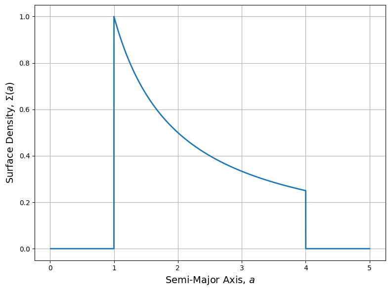
The power-law profile is called using the profile_type = 'power_law' argument, and is defined as,

\[\Sigma(a) = \Sigma_0 \left( \frac{a_\text{min}}{a} \right)^p,\]

where \(\Sigma_0\) is set using the sigma0 argument, and \(p\) is set using the power argument

power_law_profile = SigmaA(a_min=1, a_max=4, profile_type='power_law', sigma0=1, power=1)

a_vals = np.linspace(0.01, 5, 10000)
power_law_profile.plot(a_vals)

print(f"Area: {power_law_profile.compute_area():.3f}")

Area: 1.386

Gaussian Profile

The Gaussian profile is called using the profile_type = 'gaussian' argument and is defines as,

\[\Sigma(a) = \frac{\Sigma_0}{\sqrt{2\pi}\sigma} \exp{\left[ -\frac{(a - a_0)^2}{2\sigma^2} \right]},\]

where \(\Sigma_0\) is set using the sigma0 argument, \(\sigma\) is set using the gauss_width argument and \(a_0\) is set with the gauss_center argument.

Note: Since the profile is properly normalised, sigma0 also effectively sets the area under the curve.

gaussian_profile = SigmaA(a_min=1, a_max=4, profile_type='gaussian',
                          sigma0=1, gauss_center = 2.5, gauss_width = 0.3)
gaussian_profile.plot(a_vals)

print(f"Area: {gaussian_profile.compute_area():.3f}")

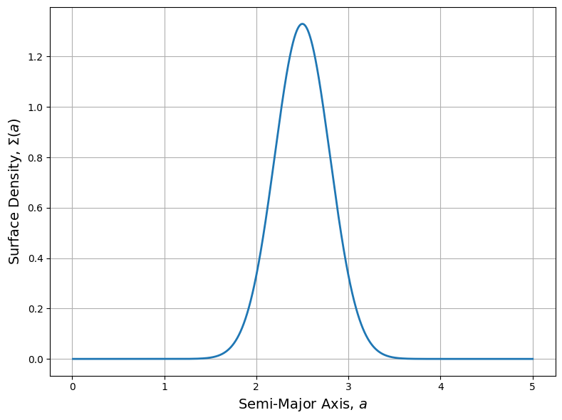
Area: 1.000

It is also possible to get truncated Gaussian profiles using this setup:

gaussian_profile_trunc = SigmaA(a_min=1.5, a_max=3.5, profile_type='gaussian',
                                sigma0=1, gauss_center = 2.5, gauss_width = 0.5)
gaussian_profile_trunc.plot(a_vals)

print(f"Area: {gaussian_profile_trunc.compute_area():.3f}")

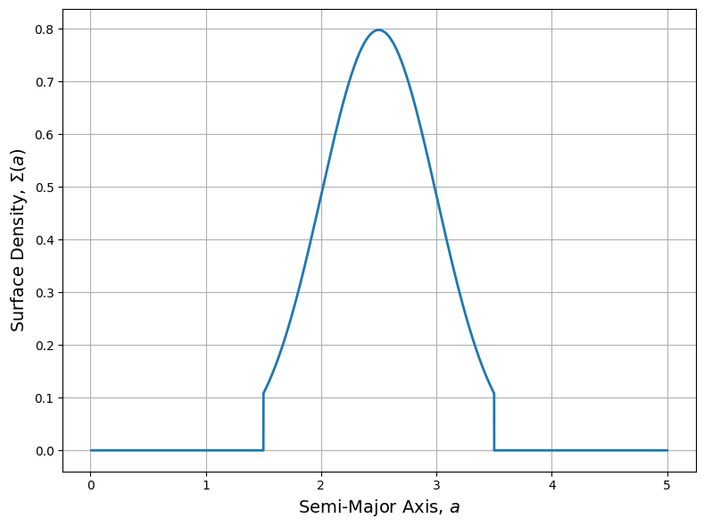
Area: 0.954

Step-Function Profile

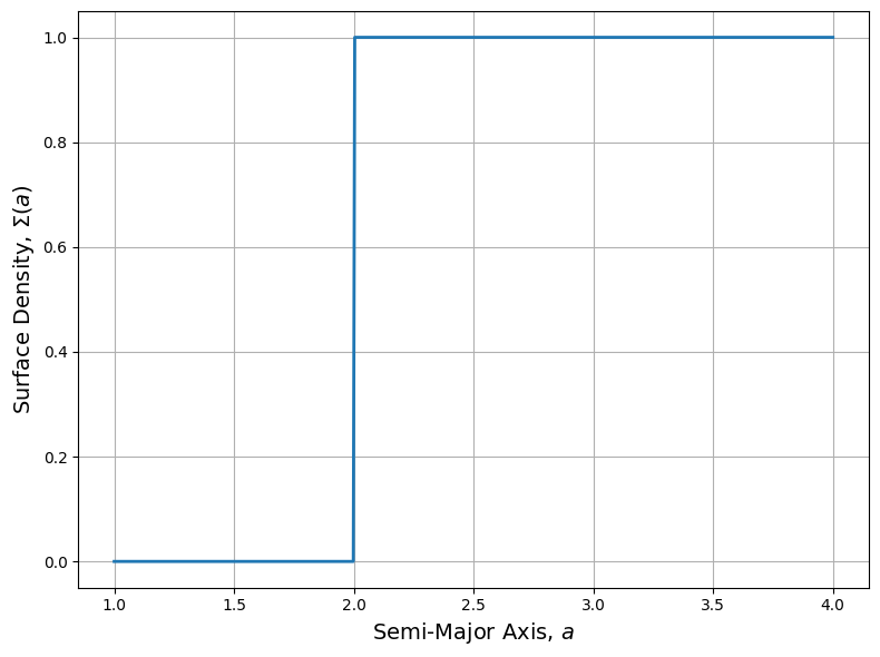
The step-function profiles are accesed by setting profile_type = 'step_up', which is defined as,

\[\Sigma(a) = \Sigma_0 \quad \text{for} \quad a > s\]

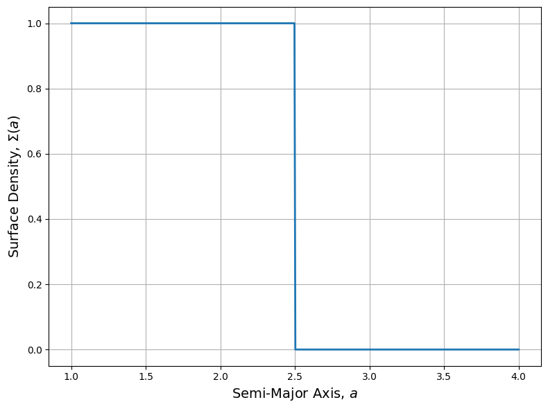
or profile_type = 'step_down', which is defined as,

\[\Sigma(a) = \Sigma_0 \quad \text{for} \quad a < s\]

In both cases, the position of the step, \(s\), is defined via the step argument.

step_up_profile = SigmaA(a_min=1, a_max=4, profile_type='step_up', step=2)
step_up_profile.plot()

step_down_profile = SigmaA(a_min=1, a_max=4, profile_type='step_down', step=2.5)
step_down_profile.plot()

Example Code (Manual Plotting)

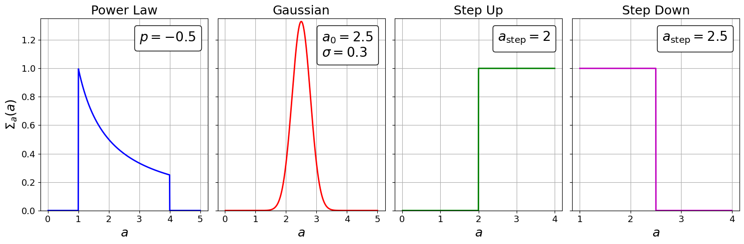
Of course, the user can choose to return the \(\Sigma(a)\) values and plot manually for full control. This is an example showing how to obtain \(\Sigma(a)\) profiles using all of the built-in methods and the plotting them together.

import matplotlib.pyplot as plt

fig, (ax1, ax2, ax3, ax4) = plt.subplots(1, 4, figsize=(15, 5))

a_vals = np.linspace(0.01, 5, 1_000)
a_vals2 = np.linspace(0.01, 4, 1_000)
a_vals3 = np.linspace(1, 4, 1_000)


# Plot data on each subplot
ax1.plot(a_vals, power_law_profile(a_vals), 'b-', lw = 2,
         label = r"$p = -0.5$")
ax1.set_title('Power Law', fontsize = 18)
ax1.set_xlabel(r'$a$', fontsize = 18)
ax1.set_ylabel(r'$\Sigma_a(a)$', fontsize = 18)

ax2.plot(a_vals, gaussian_profile(a_vals), 'r-', lw = 2,
         label = r"$a_0 = 2.5$" + "\n" + r"$\sigma = 0.3$")
ax2.set_title('Gaussian', fontsize = 18)
ax2.set_xlabel(r'$a$', fontsize = 18)

ax3.plot(a_vals2, step_up_profile(a_vals2), 'g-', lw = 2,
         label = r"$a_\mathrm{step} = 2$")
ax3.set_title('Step Up', fontsize = 18)
ax3.set_xlabel(r'$a$', fontsize = 18)

ax4.plot(a_vals3, step_down_profile(a_vals3), 'm-', lw = 2,
         label = r"$a_\mathrm{step} = 2.5$")
ax4.set_title('Step Down', fontsize = 18)
ax4.set_xlabel(r'$a$', fontsize = 18)


for ax in (ax1, ax2, ax3, ax4):
    ax.set_ylim(0, 1.35)
    ax.tick_params(axis='both', which='major', labelsize=13)
    ax.legend(fontsize = 19, loc = 'upper right', framealpha=1.0,
              edgecolor='black', handlelength=0, handletextpad=0)
    ax.grid()

for ax in (ax2, ax3, ax4):
    ax.set_yticklabels([])

plt.tight_layout()

Using a Custom Profile Type

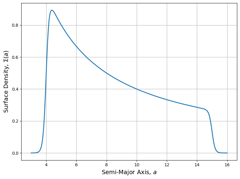
The SigmaA class can be initialised with any user-supplied function.

⚠️ Important: The supplied function should be vectorised (so scalar Python conditionals such as if/else will usually fail, use NumPy-aware operations instead), and be provided in such a way that the semi-major axis, \(a\), is the only parameter. This can be done by wrapping the function manually or using a lambda function.

# Define the custom profile
def sig_a_smooth(a, *pars):
    plaw = pars[0]
    sigma0 = pars[1]
    a_in = pars[2]
    a_out  = pars[3]
    w_in = pars[4]
    w_out = pars[5]

    f_1 = sigma0*(a_in/a)**plaw
    f_2 = 0.5*(1.0+np.tanh((a-a_in)/w_in))
    f_3 = 0.5*(1.0+np.tanh((a_out-a)/w_out))

    return f_1*f_2*f_3

parameters = [1.0, 1.0, 4.0, 15.0, 0.2, 0.2]

# Initialise the class
custom_profile = SigmaA(a_min=3, a_max=16, profile_type = 'custom',
                        sigma_func = lambda a: sig_a_smooth(a, *parameters))
custom_profile.plot()