Custom Eccentricity Distribution

In addition to the built-in eccentricity profiles, the package allows users to define and use their own custom eccentricity distributions by directly using the EccentricityDistributtion class. This feature offers maximum flexibility for experimentation and model-specific behaviour.

The way to use this class depends on whether the user-supplied function is properly normalised (this makes the computations significantly easier). Due to the increased complexity, we break this section into multiple components.

Initialising with a Normalised \(\psi_e(e,a)\) Distribution

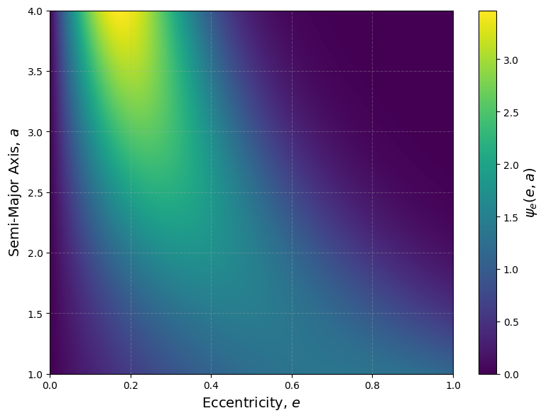
If your distribution is already correectly normalised, the process simplifies significantly. You can pass your function directly to the EccentricityDistribution class and set auto_normalise=False (default). In this case, no gridding, interpolation, or numerical integration is performed. Instead, the analytic function is stored and used directly when calculating the kernel.

See the Kernel section for how this function is evaluated during the surface density calculation.

The user must still define a_min and a_max, and may optionally specify num_e_points and num_a_points (defaults to 1000), which are used only for plotting purposes and do not affect the underlying computation.

This is the most efficient mode of operation, but should only be used if the user can guarantee that the input is correctly normalised.

from debrispy import EccentricityDistribution
import numpy as np

def normalised_rayleigh(e, a, sigma0, alpha, a_min):
    sigma = sigma0 * (a_min / a)**alpha
    return (e / sigma**2) * np.exp(-e**2 / (2 * sigma**2)) / (1 - np.exp(-1/(2*sigma**2)))

ecc_rayleigh = EccentricityDistribution(a_min=1, a_max=4,
                distribution_func=lambda e, a: normalised_rayleigh(e, a, sigma0=0.7, alpha=1, a_min=1),
                auto_normalise = False)

ecc_rayleigh.plot()

Initialising with an Unnormalised \(\psi_e(e,a)\) Distribution

If your function \(\psi_e(e,a)\) is not normalised in \(e\) for every \(a\), but you still want to use it, you can enable the auto_normalise=True flag. In this mode, the function will be automatically normalised across the eccentricity domain \([0, 1]\) at every sampled value of \(a\) via numerical integration.

In this mode, gridding becomes essential. The function must be evaluated on a 2D grid over \((e, a)\) before normalisation, and the result must be stored in a format that allows fast evaluation later. This is accomplished via interpolation, which transforms the gridded function into a callable object.

To control this behaviour, the user must specify:

1. The grid resolution: num_e_points, num_a_points (default: 1000 each)

2. The grid structure: see Gridding Options below

3. The interpolation method: see Interpolation Options below

4. The grid refinement (only for warped and adaptive grid types): grid_spread, which controls how sharply the grid adapts to features (larger values produce smoother transitions / less build up in sharp regions)

Gridding Options

When auto_normalise=True, a 2D grid is constructed over the \((e, a)\) domain. The user controls the grid using:

• num_e_points (default: 1000)

• num_a_points (default: 1000)

• grid_type (required if auto_normalise is True)

• grid_spread (default: 1.0)

Supported grid_type values include:

Grid Type	Description
'uniform'	Standard uniform grid over both \(e\) and \(a\). Best for smooth, slowly varying distributions that cover most of the range.
'warped'	Builds a grid that adapts based on the total gradient of the distribution across the entire domain. Useful for resolving sharp features aligned along the \(e\) or \(a\) axes.
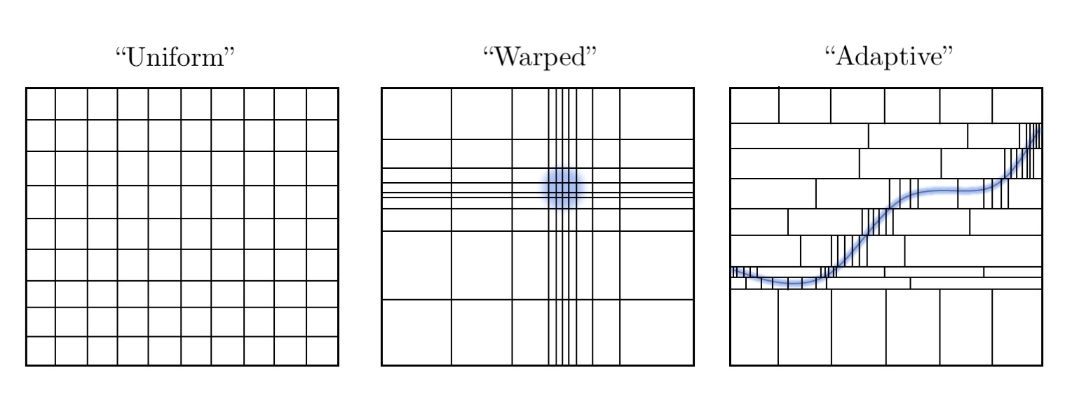
'adaptive'	Builds a per-column adaptive \(e\)-grid for each sampled value of \(a\). Ideal for handling highly localised structure or features not aligned with coordinate axes.

In all cases, the grid must be at least semi-structured in \(e\) to allow integration and normalisation. This is why fully unstructured methods like quadtrees are not supported. A schematic displaying the different grid types can be seen below, where the blue shaded parts represent steep regions.

For those interested in the details of the warping and adaptive algorithms, the implementation is fully accessible in the API and source code. See the EccentricityDistribution._create_grid method for details.

Interpolation Options

Once gridded, the normalised distribution is stored as a 2D interpolator. This is necessary for future steps when the Kernel is calculate via integration. The interpolation method is controlled via the interpolation_method argument, which supports:

• 'nearest' (for step-like functions)

• 'linear' (default and recommended for most cases)

• 'cubic' (for smooth functions, slower than linear)

Linear interpolation is typically sufficient and balances speed with smoothness. Since the grids are semi-structured by definition, we find it computationally more efficient to use scipy.interpolate.interp1d per row (i.e., per sampled value of semi-major axis).

Examples with Different Grid Types

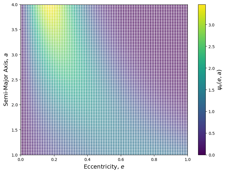
This section demonstrates the different gridding options, on purpose with a low resolution (100 points for \(e\) and \(a\)), so that it is very apparent how the grid works.

Example 1: Using uniform Grid

For smooth, slow-varying, functions a uniform grid is sufficient, and simple to compute. In this example, we consider the Rayeligh distribution.

def unnormalised_rayleigh(e, a, sigma0, alpha, a_min):
    sigma = sigma0 * (a_min / a)**alpha
    return (e / sigma**2) * np.exp(-e**2 / (2 * sigma**2))

ecc_rayleigh = EccentricityDistribution(a_min=1, a_max=4,
                    distribution_func=lambda e, a: unnormalised_rayleigh(e, a, sigma0=0.7, alpha=1, a_min=1),
                    auto_normalise = True,
                    num_e_points = 100,
                    num_a_points = 100,
                    grid_type = 'uniform',
                    interpolation_method = 'linear')

ecc_rayleigh.plot(points = True)

Example 2: Using warped Grid

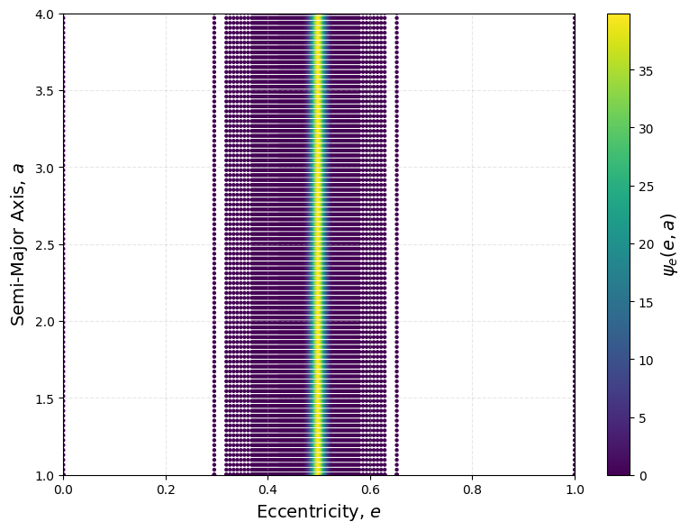
This is useful when there are sharp features aligned with one of the axes. In this example, we consider a thin Gaussian function that is centered at \(e=0.5\).

def gauss_along_a(e, a):
    return np.exp(-(e - 0.5)**2 / (2 * 0.01**2))

ecc_rayleigh = EccentricityDistribution(a_min=1, a_max=4,
                    distribution_func=gauss_along_a,
                    auto_normalise = True,
                    num_e_points = 100,
                    num_a_points = 100,
                    grid_type = 'adaptive',
                    interpolation_method = 'linear')

ecc_rayleigh.plot(points = True)

Example 3: Using adaptive Grid

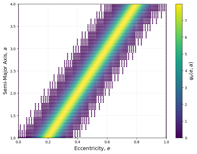
The adaptive grid takes it a step further, and thanks to a semi-structured grid, can adapt the grid points separately per :math:`a` value. As an example, we consider a Gaussian distribution, where now, the centre is no longer constant but a function of \(a\).

def gauss_along_a(e, a):
    return np.exp(-(e - 0.2*a)**2 / (2 * 0.05**2))

ecc_rayleigh = EccentricityDistribution(a_min=1, a_max=4,
                    distribution_func=gauss_along_a,
                    auto_normalise = True,
                    num_e_points = 100,
                    num_a_points = 100,
                    grid_type = 'adaptive',
                    interpolation_method = 'linear')

ecc_rayleigh.plot(points = True)

Common Functionality

The EccentricityDistribution class provides several useful methods for inspection, visualisation, and evaluation of the 2D distribution \(\psi_e(e,a)\). These are particularly helpful when auto_normalise=True, in which case the distribution is normalised numerically and interpolated.

Accessing the Distribution Values

To evaluate the distribution at specific values of eccentricity, \(e\), and semi-major axis, \(a\), one can use the distribution() method, which returns the \(\psi_e(e, a)\) values evaluated at the chosen points.

Both e and a can be scalars or NumPy arrays. If arrays are passed, broadcasting is automatically handled to return the corresponding grid of values.

• If auto_normalise=False, this directly evaluates the user-provided distribution_func(e, a).

• If auto_normalise=True, this returns interpolated and normalised values according to the chosen interpolation_method.

Note: When both \(e\) and \(a\) are scalars, the method returns a NumPy array of shape (1,) rather than a pure float. This is for consistency with the vectorised interface.

# Example of a power-law distribution
def gauss_along_a(e, a):
    return np.exp(-(e - 0.5)**2 / (2 * 0.01**2))

ecc_rayleigh = EccentricityDistribution(a_min=1, a_max=4,
                    distribution_func=gauss_along_a,
                    auto_normalise = True,
                    num_e_points = 500,
                    num_a_points = 500,
                    grid_type = 'uniform',
                    interpolation_method = 'cubic')

a_vals = np.linspace(2, 3, 5)
e_vals = np.linspace(0, 1, 5)

# This is obtained via interpolating the auto normalised distribution
dist = ecc_rayleigh.distribution(e_vals, a_vals)

print(dist)

[[0.00000000e+000 0.00000000e+000 0.00000000e+000 0.00000000e+000
  0.00000000e+000]
 [7.65392974e-135 7.65392974e-135 7.65392974e-135 7.65392974e-135
  7.65392974e-135]
 [3.98942280e+001 3.98942280e+001 3.98942280e+001 3.98942280e+001
  3.98942280e+001]
 [7.65392974e-135 7.65392974e-135 7.65392974e-135 7.65392974e-135
  7.65392974e-135]
 [0.00000000e+000 0.00000000e+000 0.00000000e+000 0.00000000e+000
  0.00000000e+000]]

Accessing the Sampled (and Normalised) Grid

The user can access the grid through the get_sampled_distribution() method. No interpolation is done on these values.

• When auto_normalise=True, this corresponds to the internal gridded data used for interpolation.

• When auto_normalise=False, the function is evaluated directly over the pre-set uniform grid (same grid used for plotting).

e_grid, a_grid, psi_grid = ecc_rayleigh.get_sampled_distribution()

2D Visualisation

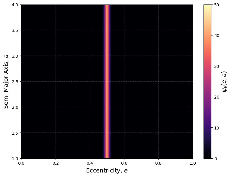
The user can visualise the 2D \(\psi_e(e, a)\) distribution as a colourmap, using the plot() method over the defined grid.

Supported keyword arguments include:

Argument	Description
log=True	Enables a logarithmic colour scale.
points=True	Visualises the distribution as scatter points rather than a continuous map.
vmin, vmax	Manually sets the colour scale limits.
save=True, filename=…	Saves the plot to the specified filename instead of displaying it.
cmap	The colourmap to use when plotting. (Default: Viridis)

ecc_rayleigh.plot(cmap = 'magma', log = False, vmin = 0, vmax = 50)

1D “Slice” Visualisation

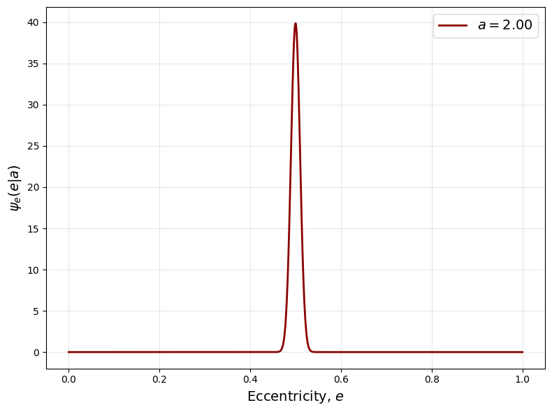
The plot_slice() method provides a convenient way to visualise 1D slices of the 2D eccentricity distribution by fixing either the eccentricity or the semi-major axis.

Usage Options:

• To plot \(\psi_e(e)\) at a fixed semi-major axis \(a\), use the fix_a keyword.

• To plot \(\psi_e(a)\) at a fixed eccentricity \(e\), use the fix_e keyword.

• Exactly one of fix_a or fix_e must be supplied.

Default Behaviour:

• 500 points are sampled by default (num_points=500).

• A new figure is created unless an existing ax is passed.

• Axis labels, a legend, and gridlines are added automatically.

• The plot is shown by default (show=True). To save instead, use save=True and specify a filename.

Customisation: The plot accepts additional matplotlib.pyplot.plot() keyword arguments. Common options include:

Argument	Description
color	Line colour
linestyle	Line style ('-', '--', ':', etc.)
marker	Marker style for points
linewidth	Thickness of the line
label	Custom legend label

ecc_rayleigh.plot_slice(fix_a = 2, num_points = 1000, linestyle = '-', linewidth = 2, color = 'darkred')

Additional Notes for auto_normalise=True

• In this case, the function is normalised along \(e\) for each sampled \(a\) and then interpolated.

• The normalisation constants, \(N(a)\) are interpolated internally, using scipy.interpolate.interp1d.

Since the resulting grid is always semi-structured (uniform, warped, or adaptive in \(e\)), we find it is computationally more efficient to use interp1 row-wise in eccentricity, rather than a fully 2D interpolator.